Sample Size and Effect Size

In this post, I show how the sample size of the treatment and control samples in an A/B test affect the impact size. The assumption here is that the population variances of both samples are known, and the responses of the individual units in these samples are Independent and Identically Distributed (IID), which simplifies this demonstration.

Setup Link to heading

Let’s say the responses in the control sample are \(X_i \sim N(\mu_X, \sigma_X^2)\) and the responses in the treatment sample are \(Y_i \sim N(\mu_Y, \sigma_Y^2)\). We want to check if the mean response of the treatment is significantly different from the mean response of the control sample (i.e. we want to check if \(\bar{Y} - \bar{X}\) is statistically different from \(0\)).

Let’s say the sample size of the control sample is \(n_X\), and the sample size of the treatment sample is \(n_Y\). We know from an older post that the distributions of these sample means are given by: \begin{align} \bar{X} \sim N(\mu_X, \frac{\sigma_X^2}{n_X}) \\ \bar{Y} \sim N(\mu_Y, \frac{\sigma_Y^2}{n_Y}) \end{align}

Effect Size Link to heading

To check whether \(\bar{Y} - \bar{X}\) is statistically different from \(0\), we’ll need the distribution of \(\bar{Y} - \bar{X}\). From another post, we know that: \begin{align} -\bar{X} \sim N(-\mu_X, \frac{\sigma_X^2}{n_X}) \end{align}

We now use the identity \(\bar{Y} - \bar{X} = \bar{Y} + (- \bar{X})\). Say \(W = (- \bar{X})\). We know that \(W \sim N(-\mu_X, \frac{\sigma_X^2}{n_X})\). For the distribution of \(\bar{Y} - \bar{X} = \bar{Y} + W\), from a standard result, we have: \begin{align} \bar{Y}-\bar{X} = \bar{Y} + W \sim N(\mu_Y-\mu_X, \frac{\sigma_Y^2}{n_Y} + \frac{\sigma_X^2}{n_X}) \tag{1} \end{align}

We now have the distribution of \(\bar{Y} - \bar{X}\). For ease of notation, let’s set \(\Delta = \bar{Y} - \bar{X}\). Given the distribution of \(\Delta\) in (1), we also can standardize it to get this result:

\begin{align} \frac{\Delta - (\mu_Y-\mu_X)}{\frac{\sigma_Y^2}{n_Y} + \frac{\sigma_X^2}{n_X}} \sim N(0, 1) \end{align}

Sample Size Selection Link to heading

The expression \(\frac{\Delta - (\mu_Y-\mu_X)}{\frac{\sigma_Y^2}{n_Y} + \frac{\sigma_X^2}{n_X}}\) is typically referred to as the test statistic. When designing an experiment, researchers typically only have control over the sample sizes chosen for the treatment and control. In addition, they’re also constrained by the total number of units available for experimentation, i.e. \(n_X + n_Y = N\).

We’d like to choose \(n_X\) and \(n_Y\) in a way that maximizes the test statistic. To derive this value, I first set \(n_X = N - n_Y\) and then take the derivative of the test statistic \(t = \frac{\Delta - (\mu_Y-\mu_X)}{\frac{\sigma_Y^2}{n_Y} + \frac{\sigma_X^2}{N - n_Y}}\) with respect to \(n_Y\):

\begin{align} \frac{\partial t}{\partial n_Y} = & -\frac{\Delta - (\mu_Y-\mu_X)}{\left(\frac{\sigma_Y^2}{n_Y} + \frac{\sigma_X^2}{N - n_Y}\right)^2} \left(-\frac{\sigma_Y^2}{n_Y^2} + \frac{\sigma_X^2}{(N - n_Y)^2} \right) = 0 \\ \implies & \left(-\frac{\sigma_Y^2}{n_Y^2} + \frac{\sigma_X^2}{(N - n_Y)^2} \right) = 0 \\ \implies & \frac{\sigma_Y^2}{n_Y^2} = \frac{\sigma_X^2}{(N - n_Y)^2} \\ \implies & \frac{\sigma_Y}{n_Y} = \frac{\sigma_X}{(N - n_Y)} \\ \implies & \frac{\sigma_Y}{\sigma_X} = \frac{n_Y}{(N - n_Y)} \\ \implies & \frac{n_Y}{N} = \frac{\sigma_Y}{\sigma_Y + \sigma_X} \\ \implies & n_Y = \frac{N\sigma_Y}{\sigma_Y + \sigma_X} \tag{2} \end{align}

In the special case where \(\sigma_Y = \sigma_X\), from (2) we have \(n_Y = n_X = N/2\). Under the assumption that both the treatment and the control samples have the same population variance, it is optimal to have both their sample sizes equal (this is why typical A/B test designs have the same number of treatment and control units).

I plot the test statistic value against the sample size \(n_Y\) for some trial values of \(\Delta, \mu_Y, \mu_X, \sigma_Y, \sigma_X \, \& \, N\) below:

import seaborn as sns
import matplotlib.pyplot as plt

# set distribution values
uy = 100 # treatment population mean
ux = 50 # control population mean
sy = 3 # treatment population standard deviation
sx = 2 # control population standard deviation 
d = 75 # delta
N = 1000 # total units available

# vary the number of treatment units
ny = [x for x in range(100, (N-100), 5)] # optimal ny = 600
# get the test statistic value
# difference between population means
ud = uy-ux
# denominator of the test statistic
s = [sy**2/ii + sx**2/(N-ii) for ii in ny]
# calculate list of test statistics
t = [(d-ud)/jj for jj in s]

# plot
sns.set(style="whitegrid")
sns.lineplot(x=ny, y=t)

# label the axes
plt.xlabel("Treatment Sample Size")
plt.ylabel("Test Statistic Value")

plt.show()

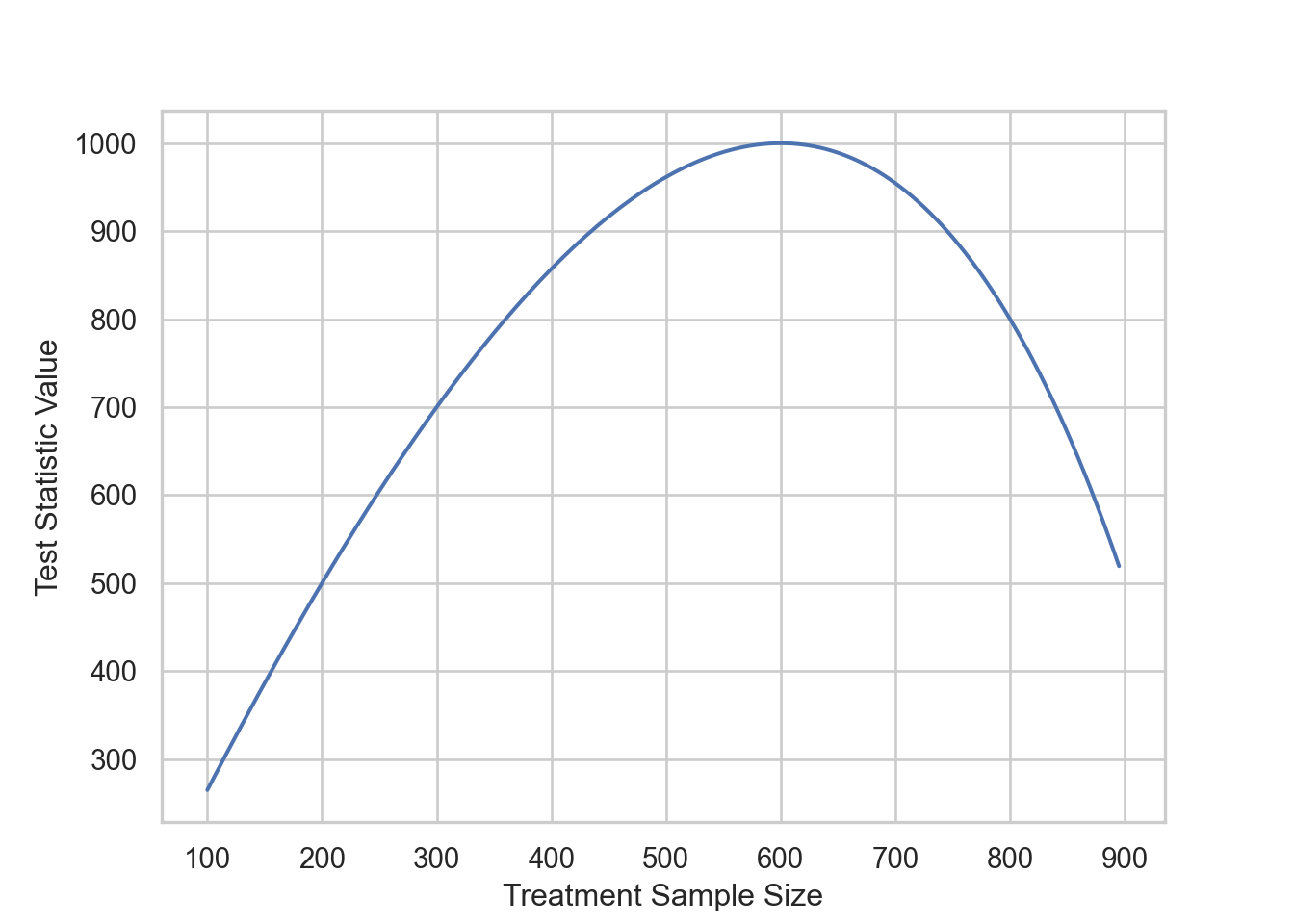
Note that for the values specified above the test statistic is maximized when \(n_Y = 600\), which is \(\frac{N\sigma_Y}{\sigma_Y + \sigma_X} = \frac{1000*3}{3+2} = 600\)